Inspired by Nerudista’s post in the Tacos de Datos website (in spanish) I asked Spotify for my data and started making some plots with them. If you want to do the same, head over to this page; once you request it, it will take a couple of days to be available. In the meantime, you can use this Google Colab, I’ve created a subset of my data for you to play with.
Among all the information you will receive, there will be some files named following this pattern: StreamingHistoryXX.json, and these are the ones we’ll use throughout this post.
The data
The files mentioned above files contain something like this:
[
  {
    "endTime" : "2019-02-04 17:14",
    "artistName" : "MGMT",
    "trackName" : "Time to Pretend",
    "msPlayed" : 261000
  },
  {
    "endTime" : "2019-02-04 17:18",
    "artistName" : "MGMT",
"..."
Where the values are:
endTime: Day and time in which a song finished, in UTC format.artistName: Name of the artist of the song.trackName: Name of the song.msPlayed: For how long (in milliseconds) a song was played.
To load these this data into a DataFrame we’ll need this tiny function:
from glob import glob
import json
import pandas as pd

def read_history():
    history = []
    for file in sorted(glob("StreamingHistory*.json")):
        with open(file) as readable:
            history.extend(json.load(readable))
    history = pd.DataFrame(history)
    history["endTime"] = pd.to_datetime(history["endTime"])
    return history

streaming_history = read_history()
streaming_history.head(5)
Which should give us something like this once we execute it:
| endTime | artistName | trackName | msPlayed | |
|---|---|---|---|---|
| 0 | 2019-02-04 17:14:00 | MGMT | Time to Pretend | 261000 |
| 1 | 2019-02-04 17:18:00 | MGMT | When You Die | 263880 |
| 2 | 2019-02-04 17:23:00 | Mr Dooves | Super Smash Bros. Brawl Main Theme (From “Super Smash Bros. Brawl”) [A Cappella] | 201518 |
Histogram.
I’ve always been a fan of the way GitHub shows developer contributions, and the data we got from Spotify seems like the perfect candidate to create something similar; however, we need to perform some transformations first.
Since we are not interested in the time each song finished we’ll get rid of the temporal part of endTime:
streaming_history["date"] = streaming_history["endTime"].dt.floor('d')Then we’ll get a count of songs per day using groupby:
by_date = streaming_history.groupby("date")[["trackName"]].count()
by_date = by_date.sort_index()
For out plot, we’ll need to know which day of the week each date refers to, we can use the properties week and weekday:
by_date["weekday"] = by_date.index.weekday
by_date["week"] = by_date.index.week
By the end, our dataframe should look like this:
| trackName | weekday | week | |
|---|---|---|---|
| date | |||
| 2019-02-04 | 5 | 0 | 6 |
| 2019-02-05 | 8 | 1 | 6 |
| 2019-02-07 | 60 | 3 | 6 |
We have almost everything we need, the next step is to get a contiuous sequence of numbers for each week. In the dataframe above the 6th week of 2016 must be the week 0, the 7th must be the week 1… I can’t think of a better way to do it than a for loop:
week = 0
prev_week = by_date.iloc[0]["week"]
continuous_week = np.zeros(len(by_date)).astype(int)
sunday_dates = []
for i, (_, row) in enumerate(by_date.iterrows()):
    if row["week"] != prev_week:
        week += 1
        prev_week = row["week"]
    continuous_week[i] = week
by_date["continuous_week"] = continuous_week
by_date.head()| trackName | weekday | week | continuous_week | |
|---|---|---|---|---|
| date | ||||
| 2019-02-04 | 5 | 0 | 6 | 0 |
| 2019-02-05 | 8 | 1 | 6 | 0 |
| 2019-02-07 | 60 | 3 | 6 | 0 |
Our next step is to generate a matrix with days ✕ weeks as dimensions, where each one of the entries will be the number of songs we listened to in that day and week:
songs = np.full((7, continuous_week.max()+1), np.nan)

for index, row in by_date.iterrows():
    songs[row["weekday"]][row["continuous_week"]] = row["trackName"]
Now we could just plot the matrix songs using seaborn:
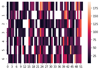
fig = plt.figure(figsize=(20,5))
ax = plt.subplot()
mask = np.isnan(songs)
sns.heatmap(songs, ax = ax)
But the result is not that great:
If we want it to look better we still need some code, the first thing to do is to clean the axis labels:
min_date = streaming_history["endTime"].min()
first_monday = min_date - timedelta(min_date.weekday())
mons = [first_monday + timedelta(weeks=wk) for wk in range(continuous_week.max())]
x_labels = [calendar.month_abbr[mons[0].month]]
x_labels.extend([
    calendar.month_abbr[mons[i].month] if mons[i-1].month != mons[i].month else ""
    for i in range(1, len(mons))])

y_labels = ["Mon", "", "Wed", "", "Fri", "", "Sun"]
The X axis labels are far more complicated than the Y ones; this is because unlike Y, the X axis is not fixed nor continuous, as such, they need to calculated based on the data. If you want a more detailed explanation, tell me in the comments or at me on twitter at @feregri_no).
After doing this we’ll perform some modifications with colours and the axis:
fig = plt.figure(figsize=(20,5))
ax = plt.subplot()
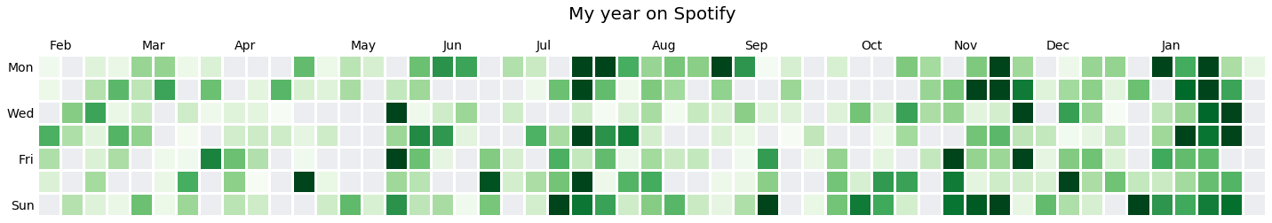
ax.set_title("My year on Spotify", fontsize=20,pad=40)
ax.xaxis.tick_top()
ax.tick_params(axis='both', which='both',length=0)
ax.set_facecolor("#ebedf0")
fig.patch.set_facecolor('white')And finally, we can use seaborn’s heatmap again, this time with a few extr arguments that I will explain later:
sns.heatmap(songs, linewidths=2, linecolor='white', square=True,
            mask=np.isnan(songs), cmap="Greens",
            vmin=0, vmax=100, cbar=False, ax=ax)

ax.set_yticklabels(y_labels, rotation=0)
ax.set_xticklabels(x_labels, ha="left")
The arguments are as follows:
songs: our matrix with shapedays ✕ weekswith the counts of songs per day,linewidths: the size of the spacing between each patch,linecolor: the colour of the spacing between each patch,square: this tells the function that we want to keep the aspect ratio1:1for each patch,mask: a very interesting argument, it will help us “mask” the patches for which there is no recorded value, this argument should be a boolean matrix of the same dimensions as the data being plotted, where eachTruemeans that that specific value must be masked,cmap: the colormap to be used, luckily for us, the value “Greens” matches with the colour palette chosen by GitHub,vmin: the value that should be considered as the minimum among our values,vmax: the value that should be considered as the maximum among our values, I’d consider 100 to be the maximum, even though my record sits as 190 in a day!cbar: a boolean value to indicate whether we want to show the colour bar that usually comes with the heatmap,ax: the axes our plot should be plotted on.
And voilà, our plot is ready:
It is up to you to modify the plot, may be by adding information about the number of songs, or show the colorbar… a great idea would be to recreate this plot in a framework such as D3.js, but that may well belong to another post. Again, feel free to head over to this Colab and contact me via twitter @feregri_no.
